Lotka-Volterra Equations for Modelling Population Dynamics

1. Predator-Prey Equations

Theory

The Lotka-Volterra predator-prey equations are a pair of first order nonlinear differential equations used to describe the population dynamics of the interaction between a predator species and a prey species. It is a relatively simplified model which makes several assumptions about the environment and the evolution of each population. The prey is assumed to have an unlimited food supply and reproduce exponentially unless preyed upon. The food supply of the predators depends entirely on the size of the prey population, and predators have limitless appetite. During the process, the environment does not change, and there is no natural selection in either population. Both populations change naturally at a rate proportional to population size.

Model

Equations

The predator-prey population dynamics are represented by the pair of equations[^1]:

$$\frac{dx}{dt} = \alpha x - \beta xy$$

$$\frac{dy}{dt} = \delta xy - \gamma y$$

where x is the number of prey, y is the number of predators, and α, β, δ, γ are constant values that represent growth, predation, and death rates.

Parameters

In the prey equation, α represents the intrinsic growth rate of the prey population, and β represents the rate at which prey die to predation. In the predator equation, δ represents the rate of population increase after consuming prey, and γ represents the intrinsic death rate of the predator population. Given these parameters, the prey equation can be understood as “the rate of population change depends on the intrinsic growth rate minus the rate of predation,” while the predator equation can be understood as “the rate of population change depends on the rate of prey consumption minus the intrinsic death rate.” In a real-world situation, β and δ are not the same value, since predators typically do not reproduce at the same rate at which they consume prey.

To model a hypothetical predator-prey interaction, the following parameters were chosen:

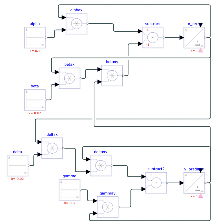
α = 0.1, β = 0.02, δ = 0.02, γ = 0.3, x(0) = 10, y(0) = 10

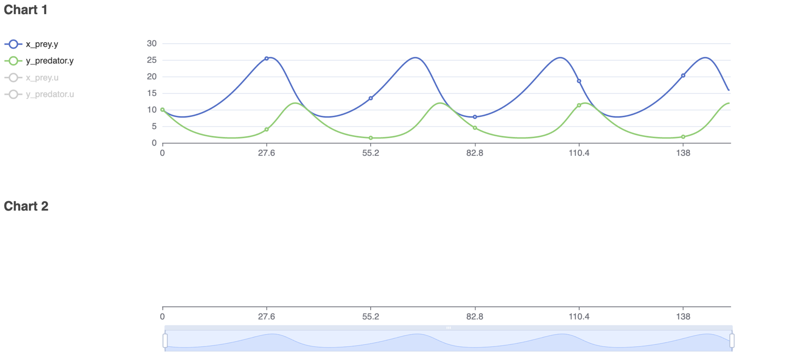
This interaction was modeled for 150 units of time using Physhub, and the resulting diagram and charts are attached below (Fig.1, Fig.2).

Results

The equations have periodic solutions which continue indefinitely, given that the initial assumptions are true. The resulting chart shows the distinct repeating curves of both populations. The maximum and minimum values of the predator equation follow those of the prey equation by a fixed delay. At time 0, the number of prey is not enough to sustain the number of predators. The predator population decreases significantly, while the prey population begins to increase due to a lack of predation. As the prey population increases, the predators have more food, and thus their population begins slowly increasing. At a certain point, the prey are being hunted at a higher rate than they can reproduce, and their population begins to decrease, restarting the cycle.

References

2. Competition Equations

Theory

The Lotka-Volterra model of interspecific competition describes the dynamics of two populations of different species that compete for the same resource. This model demonstrates an important ecological concept, the competitive exclusion principle. Stated simply, if there are two species whose resource pools overlap too much, one species will outcompete the other and exclude it from the resource pool. The model consists of a pair of differential equations which build off the basic logistic model. The logistic model focuses on competition between individuals of the same species ((intraspecific)), while the Lotka-Volterra equations incorporate a competition coefficient to model competition between individuals of different species ((interspecific)).

Model

Equations

This model of interspecific competition is represented by two equations[^2]:

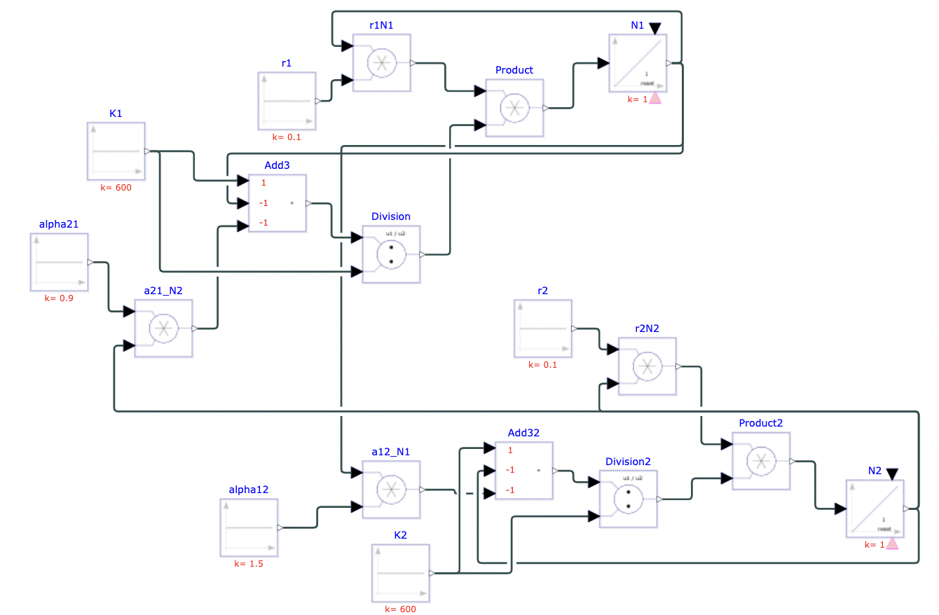
$$\frac{dN_{1}}{dt} = r_{1}N_{1}(\frac{K_{1} - N_{1} - \alpha_{21}N_{2}}{K_{1}})$$

$$\frac{dN_{2}}{dt} = r_{2}N_{2}(\frac{K_{2} - N_{2} - \alpha_{12}N_{1}}{K_{2}})$$

where $N_{1}$ and $N_{2}$ are populations of two different species, $K_{1}$ and $K_{2}$ are the carrying capacity of the two populations, and r and α are constants.

Parameters

N represents the existing population at a given time; K is the carrying capacities, or the maximum population the environment can support. r is the per capita growth rate, which is the rate of population change per existing individual. α is the competition coefficient, which measures the competitive effect of one species on another. In this model, $\alpha_{21}$ represents the effect of species 2 on species 1, hence the notation “21.” Similarly, $\alpha_{12}$ represents the effect of species 1 on species 2. The equations build off the simpler logistic growth equation, $\frac{dN}{dt} = rN(\frac{K - N}{K})$. The main difference is the addition of the $- \alpha N$ term, which represents the competitive effect of one species on the other per individual. For example, a moose (species 1) who consumes three times the amount of resources a deer (species 2) consumes would have an $\alpha_{12}$ of 3.0. However, $\alpha_{12}$ and $\alpha_{21}$ are usually not reciprocal values. The moose and deer likely both consume resources that the other does not, which changes their competitive effects on each other. In general, an α-value greater than 0 indicates that there is some overlap in resource utilization.

To model a hypothetical instance of interspecific competition, the following parameters were chosen:

$N_{1} = 100$, $N_{2} = 100$, $K_{1} = 600$, $K_{2} = 600$,
$r_{1} = 0.1$, $r_{2} = 0.1$, $\alpha_{21} = 0.9$, $\alpha_{12} = 1.5$.

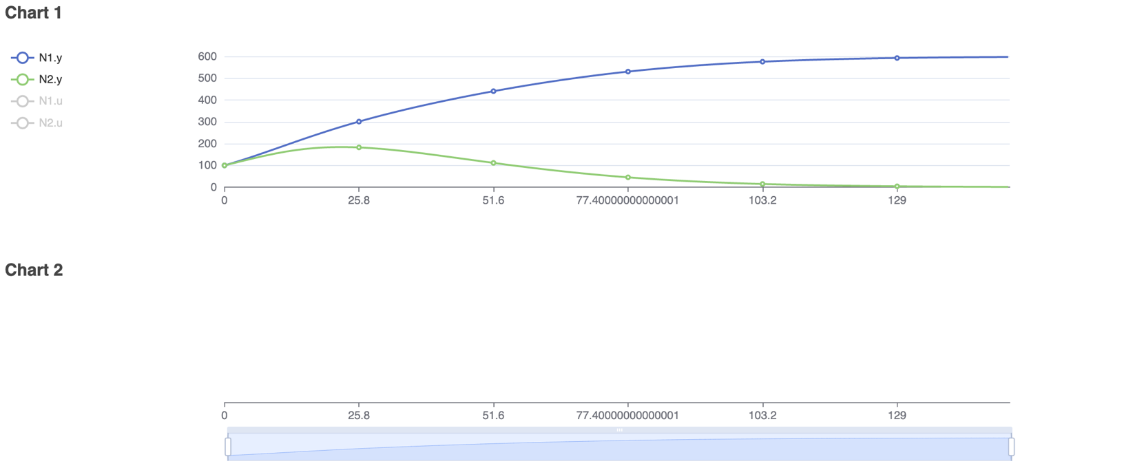
The interaction was modeled for 150 units of time using Physhub, and the resulting diagram and charts are below (Fig.3, Fig.4).

Results

In the parameters, the only difference between the two species was their competitive effects: species 1 has a greater effect on species 2, and it eventually outcompetes species 2. Both species exhibit initial growth, but the population of species 2 quickly begins to decrease. The population of species 1 increases continuously, but at a slower rate than if species 1 was not present. Eventually, because species 1 outcompetes and excludes species 2, the population of species 1 will increase to carrying capacity, while species 2 will eventually reach local extinction in this environment.

References

[^1]: [Weisstein, Eric W.] "Lotka-Volterra Equations." From [MathWorld]--A Wolfram Web Resource. [https://mathworld.wolfram.com/Lotka-VolterraEquations.html]

[^2]: “Quantifying Competition Using the Lotka-Volterra Model.” 2022. June 17, 2022. https://bio.libretexts.org/@go/page/83719.