SIRS Model
Theory
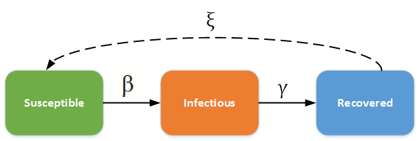
The SIRS ((susceptible-infectious-recovered-susceptible)) model is a compartmental model that is closely related to the more basic SIR model. It uses the same three compartments, but there is now an additional constant. The movement of individuals from susceptible to infectious to recovered is identical to that of the SIR model; however, once individuals recover, their immunity decreases over time, and they eventually re-enter the susceptible compartment.
The constants ß and γ follow the same concept as in the SIR model. The new constant, ξ, is the rate at which recovered individuals become susceptible again, or the rate of immunity loss. Assuming a closed population and non-fatal disease, the disease will persist in the population at a low but relatively stable proportion. This model can be applied to diseases in which immunity wanes over time, such as the common cold or seasonal influenza.
Model
Equations
This model is represented by a set of three differential equations^1:
$$\frac{dS}{dt} = \frac{- ßSI}{N} + \xi R$$
$$\frac{dI}{dt} = \frac{ßSI}{N} - \gamma I$$
$$\frac{dR}{dt} = \gamma I - \xi R$$
where S = number of susceptible individuals, I = number of infectious individuals, R = number of recovered individuals, ß = rate of infection ((constant)), [γ = rate of recovery ((constant)), ξ]{.mark} = rate of immunity loss ((constant)), and N = S + I + R = total population ((constant)).
Parameters
In the SIRS model, the constants ß, γ, and N follow the same concepts as in the SIR model. ξ is calculated by taking the reciprocal of the average duration of immunity.
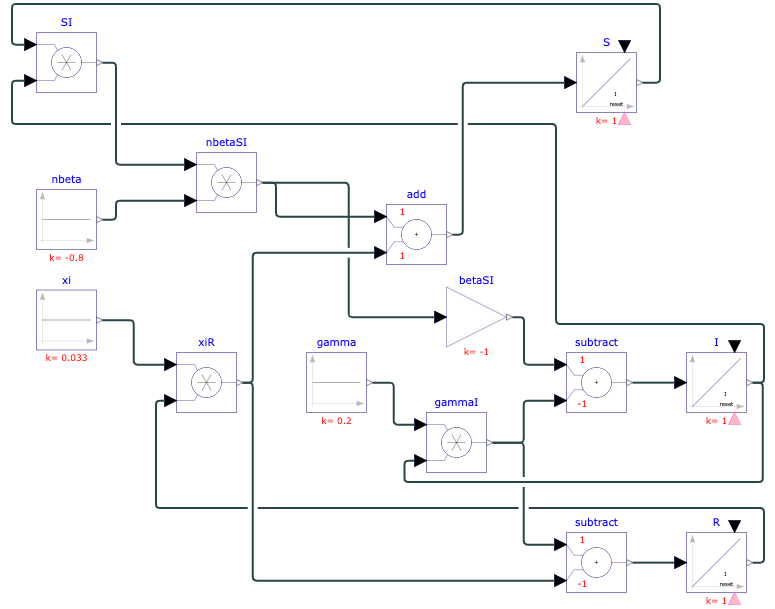
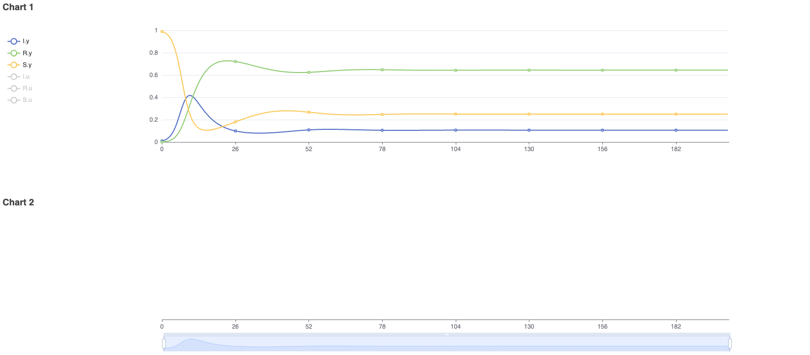
To model real-life diseases, ß, γ, ξ, and N are selected to match the situation. For example, a highly infectious, non-fatal disease that appears in a closed population of 1, or 100%, has an infection rate of 0.8, a recovery rate of 0.2, and immunity is lost at a rate of 0.033. The resulting model predicts the behavior of the disease over a selected period. The figures below show the diagram created in Physhub and the corresponding charts ((Fig.1, Fig.2)).
Results
The model successfully simulates the changes in the number of susceptible, infectious, and recovered individuals in a closed population over time. The simulation was run for 200 units of time. As predicted in theory, the number of individuals in each compartment leveled out after initial fluctuations. In general, this model accurately simulates infectious disease behavior and compartmental changes in a population given any set of realistic parameters.
SEIR Model

Theory
The SEIR ((susceptible-exposed-infectious-recovered)) model is another useful compartmental model for infectious diseases. It is slightly more complex than the SIR model, involving an additional compartment and constant parameter. In this model, individuals are born with no immunity ((susceptible)) and encounter the disease at some point. Instead of immediately becoming infectious, there is an incubation period where individuals have been exposed but are not yet infectious. After a certain amount of time, individuals then move to the infectious compartment. Individuals who recover gain total immunity and are unable to contract the disease again. The constants ß and γ follow the same concept as in the SIR model. The new constant, σ, is the rate at which exposed individuals become infectious, or the incubation rate. Assuming a closed population and a non-fatal disease, all susceptible individuals will become infectious and eventually recover. This model is typically applied to diseases with a distinct incubation period, such as chicken pox, dengue fever, and even certain cases of COVID-19.
Model
Equations
This model is represented by a set of four differential equations^2:
$$\frac{dS}{dt} = \frac{- ßSI}{N}$$
$$\frac{dE}{dt} = \frac{ßSI}{N} - \sigma E$$
$$\frac{dI}{dt} = \sigma E - \gamma I$$
$$\frac{dR}{dt} = \gamma I$$
where S = number of susceptible individuals, E = number of exposed individuals, I = number of infectious individuals, R = number of recovered individuals, ß = rate of infection ((constant)), [γ = rate of recovery ((constant))], σ = rate of incubation ((constant)), and N = S + E + I + R = total population ((constant)).
Parameters
In the SEIR model, the constants ß, γ, and N follow the same concepts as in the SIR model. σ is calculated by taking the reciprocal of the average duration of incubation.
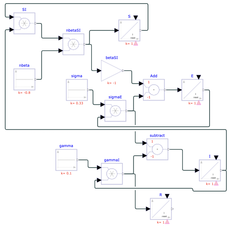
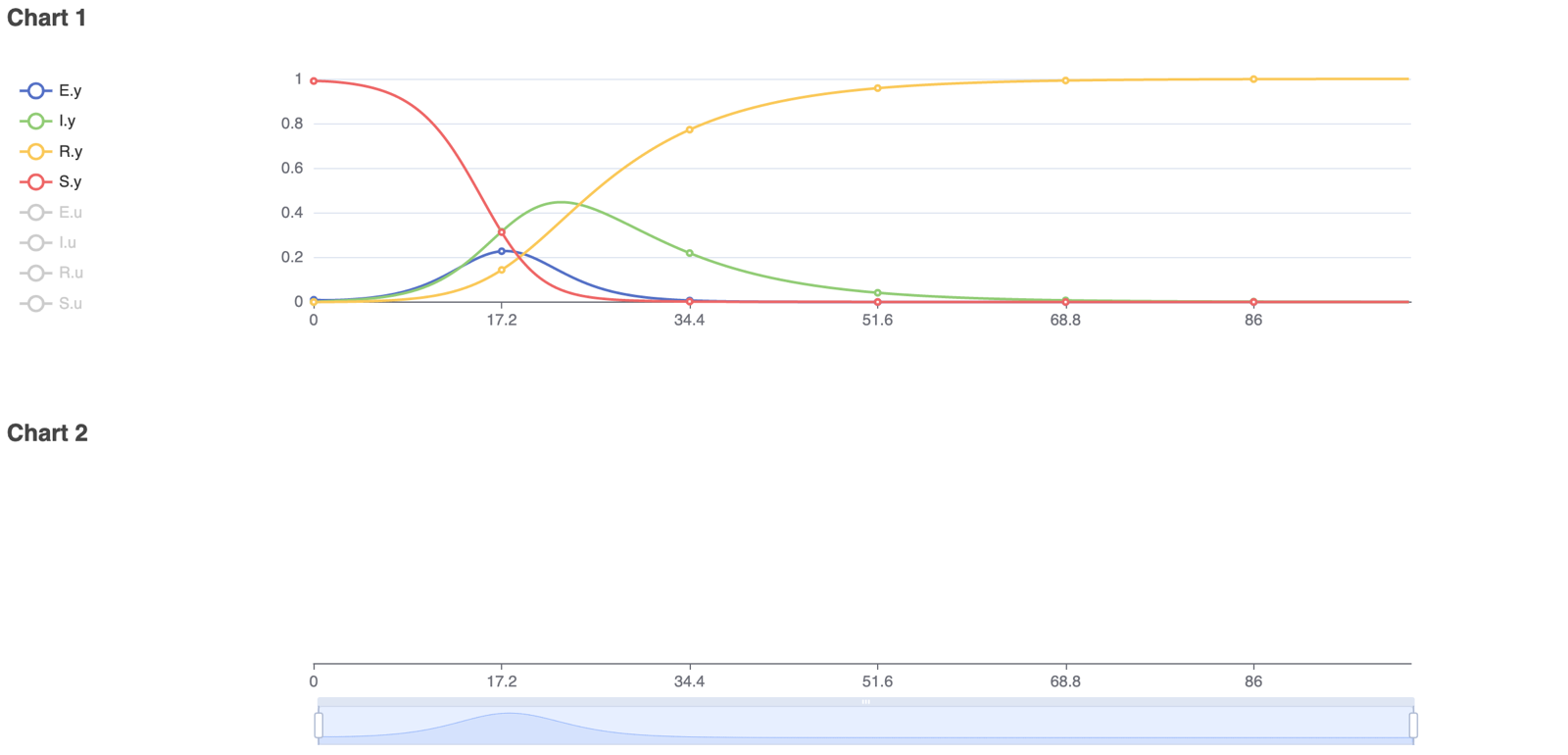
To model real-life diseases, ß, γ, σ, and N are selected to match the situation. For example, a highly infectious, non-fatal disease that appears in a closed population of 1, or 100%, has an infection rate of 0.8, an incubation rate of 0.33, and a recovery rate of 0.1. The resulting model predicts the behavior of the disease over a selected period. The figures below show the diagram created in Physhub and the corresponding charts ((Fig.3, Fig.4)).
Results
The model successfully simulates the changes in the number of susceptible, exposed, infectious, and recovered individuals in a closed population over time. The simulation was run for 100 units of time. As predicted in theory, all individuals became exposed or infectious and eventually recovered. In general, this model accurately simulates infectious disease behavior and compartmental changes in a population given any set of realistic parameters.
